-
Introduced in DeepSeek v2, https://arxiv.org/pdf/2405.04434
-
pytorch implementation https://github.com/fla-org/flash-linear-attention/blob/main/fla/layers/mla.py
-
MLA utilizes low-rank key-value joint compression to eliminate the bottleneck of inference-time key-value cache.
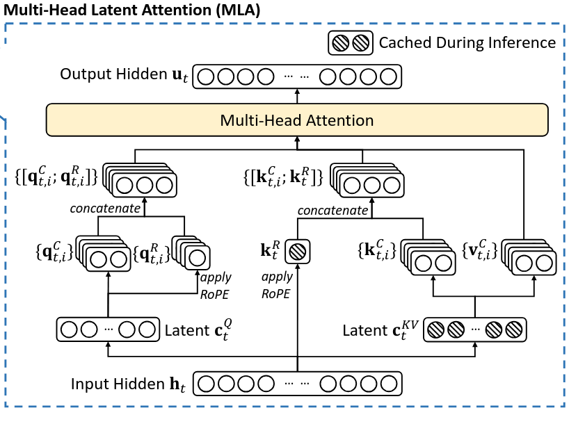
Full Formula of MLA
- Notation:
- is an down-projection matrix to the compressed space
- is an up-projection matrix from the compressed space
Setup and dimensions
Let
- =
hidden_dim - =
num_attention_heads - =
qk_nope_head_dim(no-PE/low-rank per-head dim) - =
qk_rope_head_dim(RoPE per-head dim) - =
q_lora_rank - =
kv_lora_rank
Vectors (columns):
- ,
- Per head : , , , ,
Matrices (biases omitted; matrices left-multiply column vectors):
- (code:
q_down_lora) - (code:
q_up_nope) - (code:
q_up_rope) - (code:
kv_down_lora) - (code:
k_up_nope) - (code:
k_rope) - (code:
v_up) - (code:
out_proj)
RoPE preserves size: .
Algorithm
where the boxed vectors in blue need to be cached for generation.
Inference optimization
-
During inference, the naive formula needs to recover and from for attention.
-
Fortunately, due to the associative law of matrix multiplication, we can absorb into , and into .
- Proof below
- Through this optimization, we avoid the computational overhead for recomputing and during inference.
-
The absorption trick means that head dimension for self-attention is () during inference, compared to () during training.
- Given that for DeepSeek-V2, is set to and is set to , then the reduction dimension is about times during inference
- Thus, we’re trading off KV-cache size for arithmetic intensity
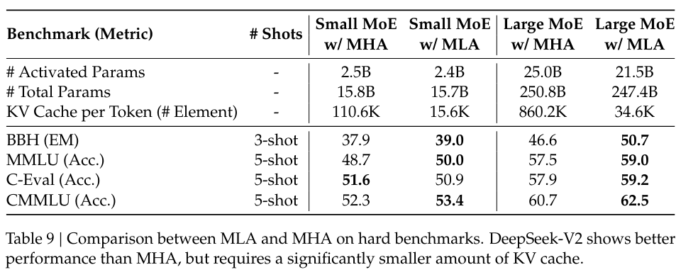
KV cache per token
| Attention Mechanism | KV Cache per Token (# Element) | Capability |
|---|---|---|
| Multi-Head Attention (MHA) | Strong | |
| Grouped-Query Attention (GQA) | Moderate | |
| Multi-Query Attention (MQA) | Weak | |
| MLA (Ours) | Stronger |
denotes the number of attention heads, denotes the dimension per attention head, denotes the number of layers, denotes the number of groups in GQA, and and denote the KV compression dimension and the per-head dimension of the decoupled queries and key in MLA, respectively.
The amount of KV cache is measured by the number of elements, regardless of the storage precision. For DeepSeek-V2, is set to and is set to . So, its KV cache is equal to GQA with only 2.25 groups, but its performance is stronger than MHA.
Ablations between MQA, GQA, MHA, and MLA
Inference optimizations - Absorption
Multi-Head Latent Attention (MLA) — Inference Absorption Proof
- They key to the proof is to do it on a per-head basis
MLA equations (condensed)
Per-head scaled scores use :
Claim A (keys): absorb into the query side
For head , the no-PE part of the dot product is
Define the composed matrix and the KV-space query
Then
Consequence. During inference, you only need the cached (not ). Precompute once and form for the current token. The total score for head becomes
(If you prefer a single matrix, stack the blocks: .)
Claim B (values): absorb into the output projection
Let be the attention weights per head. Then where we defined the compressed-space mixture
Stack across heads into and set . The final output is
Consequence. Precompute . At inference you never materialize or :
- build directly in the compressed space from cached and weights ,
- concatenate to , and
- apply once to get .
What to cache (matches the blue boxes)
- for each past token — the low-rank KV cache.
- (per head or shared), unchanged by the trick.
No need to cache or recompute or .
Optimized inference recipe (per new token )
- Compute , , and (cache ).
- For each head , compute .
- Scores: .
- Weights: .
- Mix in compressed space: .
- Output: .
All expensive per-token operations after step 1 happen in the low-rank space.
Code to absorb into
- PR for absorbing w_uk into w_O https://github.com/deepseek-ai/DeepSeek-V3/pull/702
- As before, important to reshape the weights on a per-head basis to absorb correctly
import torch
from torch import nn

class AbsorbDemo:

    def __init__(self, bsz=1, q_len=1, kv_len=4, dim=7168, kv_lora_rank=512, n_heads=128, v_head_dim=128):

        self.n_heads = n_heads
        self.v_head_dim = v_head_dim
        self.dim = dim

        self.scores = torch.rand(bsz, q_len, n_heads, kv_len)
        self.kv_cache = torch.rand(bsz, kv_len, kv_lora_rank)
        self.w_uv = torch.rand(n_heads, v_head_dim, kv_lora_rank)
        self.wo = nn.Linear(self.n_heads * self.v_head_dim, self.dim, bias=False)
        self.wo_absorb = None

    def run(self, absorb=False):
        x = torch.einsum("bsht,btc->bshc", self.scores, self.kv_cache)
        if absorb:
            if self.wo_absorb is None:
                wo = self.wo.weight
                wo = wo.transpose(0,1).view(self.n_heads, self.v_head_dim, self.dim)
                self.wo_absorb = torch.einsum("hdc,hdi->hci", self.w_uv, wo)
            x = torch.einsum("bshc,hci->bshi", x, self.wo_absorb)
            x = torch.sum(x, dim=2)
        else:
            x = torch.einsum("bshc,hdc->bshd", x, self.w_uv)   # it cost large memeory
            x = self.wo(x.flatten(2))
        return x


demo = AbsorbDemo()
tensor1 = demo.run(absorb=False)
tensor2 = demo.run(absorb=True)
print("w/o absorb:", tensor1.data)
print("w   absorb:", tensor2.data)
print(torch.allclose(tensor1.data, tensor2.data, atol=1e-03))
MLA Absorption: Why it’s an Inference-Only Optimization
Short answer: It’s great for generation-time reuse (weights frozen; KV cache grows), but awkward or counter-productive for training because of autograd dependencies and compute shape. In the absorbed path the QK reduction per head is , whereas in the canonical training path it’s . The inference win is from never materializing or recomputing and over the growing cache, not from a smaller reduction dimension.
Why inference-only (autograd + compute)
-
Autograd dependency.
The absorbed matrices are products of learnable weights: and . If you precompute/cache these as constants for speed, then in the graph they don’t depend on , so gradients vanish: . That’s fine in eval, but during training it kills learning.You could keep in-graph (no detach) so the chain rule applies: and (and similarly for ). But then you must rebuild these products every forward, keep intermediates for backward, and backprop through extra large matmuls—negating the intended speed/memory win.