- We can horizontally partition the computation for one tensor operation across multiple devices, named Tensor parallelism (TP).
Summary
-
Normal GEMM is (`batch x in_features) x (in_features x out_features)
- output is
(batch x out_features)
- output is
-
column-linear
- weight matrix is sharded by the columns (i.e. by the out_features dimension)
- input is not sharded
- GEMM on rank i: (`batch x in_features) x (in_features x out_features/world_size)
- output is
(batch x out_features/world_size) - output is sharded by the out_features dimension but correct
- no communication needed (except a gather if we’re at the end)
-
row-linear
- weight matrix is sharded by the rows (
in_featuresdimension) - input is sharded by the rows (i.e. by the
in_featuresdimension) - GEMM on rank i: (`batch x in_features / world_size) x (in_features/world_size x out_features)
- output is
(batch x out_features) - we need to all reduce to obtain the correct output
- `output = all_reduce(output, tp_group)
- weight matrix is sharded by the rows (
Derivations
- We write the derivations by splitting in two, however in general, the matrixes are split equally within the GPUs in a given node
Parallelizing a GEMM (General Matrix multiply)
-
is , A is $d_{model} \times d_{hidden}$$
-
First option (parallelize and aggregate, each “thread” computes a matrix of the same dimension as ) (more memory efficient, but requires all_reduce at the end): - split along its rows and input along its columns: - , - is and is - Then, (it’s true, I checked) - intuition: - A matrix-matrix mul can be seen as multiple matrix-vector mul concatenated (along the columns of A). - In such matrix-vector mul, each element of a given column in is responsible for picking out its corresponding column in , mutliply it by itself, and then the result is summed to obtain the new column in - Here, we parallelize the computation over these columns, and aggregate at the end
-
Second option (parallelize and concatenate, each “thread” produces a slice of ) (less memory efficient but no synchronization):
- Split along its columns
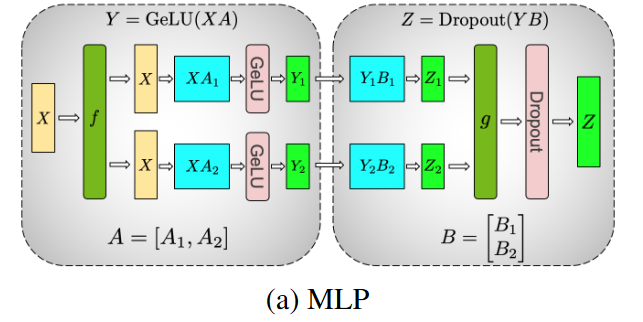
MLP
-
is , A is , B is
-
Usual two-layer MLP block is
- Y =
- i.e. one GEMM (general matrix multiply)
- one GeLU
- one GEMM
-
Parallelizing the
-
First option (parallelize and aggregate, each “thread” computes a matrix of the same dimension as ):
-
- GeLU is nonlinear, so
- Thus we need to sychnronize before the GeLU function
- GeLU is nonlinear, so
-
Second option (parallelize and concatenate, each “thread” produces a slice of ):
- Split along its columns
-
This partitioning allows the GeLU nonlinearity to be independently applied to the output of each partitioned GEMM
-
This is advantageous as it removes a synchronization point
-
-
Parallelizing
- Given we receive = , split by the columns, we split by its rows
- Compute
- Synchronization
- Z =
all_reduce(Y_iB_i)by summing them - Called in the diagram
- Z =
-
Diagram
- is an all-reduce in the forward where the matrix are aggregated by summing, identity (or splitting) in the backward
- is an identity (or splitting) in the forward, and an all-reduce in the backward
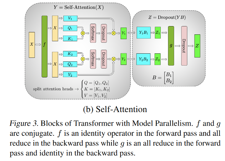
Self-Attention
-
They exploit inherent parallelism in the multihead attention operation.
-
partitioning the GEMMs associated with key (K), query (Q), and value (V ) in a column parallel fashion such that the matrix multiply corresponding to each attention head is done locally on one GPU
-
This allows us to split per attention head parameters and workload across the GPUs, and doesnt require any immediate communication to complete the self-attention.
-
The subsequent GEMM from the output linear layer (after self attention) is parallelized along its rows (i.e. ), given it receives the self-attention split by columns, by design (requiring no communication)
-
Finally, we apply , the all_reduce to obtain the result (before dropout)
-
-
Diagram