Scaling Laws for Batch Size

“An Empirical Model of Large-Batch Training”

Takeaways

• The gradient noise scale (essentially a measure of the signal-to-noise ratio of gradient across training examples) predicts the largest useful batch size across many domains and applications

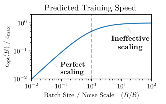
• Best-tradeoff for efficiency is to select $B={\mathcal{B}}_{noise}$

• Noise scale growth over training: $\mathcal{B}$ will grow when the gradient decreases in magnitude, as long as the noise $tr(\Sigma )$ stays roughly constant. Since $|G|$ decreases as we approach the minimum of a smooth loss, we would expect B to increase during neural network training.

  • The optimal learning rate initially scales linearly as we increase the batch size. For Adam and RMSProp, the optimal learning rate initially obeys a power law $ϵ(B)\sim B^{\alpha }$ with $\alpha$ between $0.5$ and $1.0$ depending on the task,
  • Early in training, smaller batches are sufficient to make optimal progress, while larger batches are required later in training.

• Why it matters:

  • A major enabler in the growth of DL has been parallelism – the extent to which a training process can be usefully spread across multiple devices. Regardless of how much total computation is available, if model training cannot be sufficiently parallelized, then it may take too much serial time and therefore may be practically infeasible
    • Common source of parallelism: data parallelism
    • Large batch sizes can achieve almost linear speed-ups in training without substantially harming sample efficiency or generalization.

• Why is there an optimal batch size?

  • Set up: SGD optimization
  • If batch size very small
    • The gradient approximation will have very high variance, and the update will be mostly noise
    • Over many updates, the noise will wash out
    • However, this requires many sequential steps
    • We can get a linear gain in efficiency by parallelizing i.e. increasing the batch size and get an equivalent results, by aggregating those small updates and applying them all at once (by increasing batch size and learning rate)
  • If batch size very big
    • The gradient approximation is equal to the true gradient
    • However, reducing the batch size by two will likely give us the same approximation
    • Thus, we’re using twice as much computation for little gain
  • The optimal batch size gives us a good (not too noisy) gradient approximation, while being compute efficient.

• Smaller batch size may helpful to escape local minimas, as the noise in the estimated gradient will get us out of it

Definition of gradient noise scale

Summary

• Gradient noise scale ${\mathcal{B}}_{noise}\approx \frac{tr(\Sigma )}{|G{|}^2}$ = the noise scale is equal to the sum of the variances of the individual gradient components, divided by the global norm of the gradient
• The optimal improvement of the loss from the noisy gradient update is a function of ${\mathcal{B}}_{noise}$ and $B$ i.e. $\Delta L_{opt}(B)=\frac{\Delta L_{max}}{1+{\mathcal{B}}_{noise}/B}$
• In this way, we can compute when we get diminishing returns from increasing batch size, the conclusion is that batch size should roughly equal the noise scale
  • 

Detailed

• Consider a model, parameterized by variables $\theta$, whose performance is assessed by a loss function $L(\theta )$. The loss function is given by an average over a distribution $\rho (x)$ over data points $x$. Each data point $x$ has an associated loss function $L_x(\theta )$, and the full loss is given by $L(\theta )={\mathbb{E}}_{x\sim \rho }[L_x(\theta )]$

• The true gradient is $G(\theta )=\nabla L(\theta )$

• Estimated gradient: $G_{est}(\theta )=\frac{1}{B}{\sum }_{i=1}^B{\nabla }_{\theta }{L}_{x_i}(\theta );x_i\sim \rho$

• $G_{est}(\theta )$ is a random variable such that

  • $\mathbb{E}[G_{est}(\theta )]$ = $G(\theta )$
  • $cov(G_{est}(\theta ))=\frac{1}{B}\Sigma (\theta )$
    • where the per-example covariance matrix of the gradient $\Sigma (\theta )=co{v}_{x\sim \rho }({\nabla }_{\theta }{L}_x(\theta ))={\mathbb{E}}_{x\sim \rho }[({\nabla }_{\theta }{L}_x(\theta ))({\nabla }_{\theta }{L}_x(\theta ){)}^T]-G(\theta )G(\theta {)}^T$

• We are interested in how useful the gradient is for optimization purposes as a function of $B$, and how that might guide us in choosing a good $B$.

• We can do this by connecting the noise in the gradient to the maximum improvement in true loss that we can expect from a single gradient update.

• Letting $G$ and $H$ be the true gradient and hessian at parameters $\theta$

  • We can perturb the parameters $\theta$ by a small vector $V$ to $\theta -ϵV$, where $ϵ$ is the step size
  • We do a quadratic Taylor expansion of the loss around this perturbation
    • $L(\theta -ϵV)=L(\theta )-ϵG^{T}V+\frac{1}{2}{ϵ}^2{V}^{T}HV$
  • Now if we replace $V$ by $G_{est}$, we get on expectation
    • $\mathbb{E}[L(\theta -ϵG_{est})]=L(\theta )-ϵ|G{|}^2+\frac{1}{2}{ϵ}^2(G^{T}HG+\frac{tr(H\Sigma )}{B})$
    • for the trace term, remember that the scalar $\mathbb{E}[G_{est}^T{G}_{est}]=tr(\Sigma )$
  • Let’s minimize this equation w.r.t $ϵ$
    • $\frac{d}{dϵ}\mathbb{E}[L(\theta -ϵG_{est})]=-|G{|}^2+ϵ(G^{T}HG+\frac{tr(H\Sigma )}{B})$
    • ${ϵ}_{opt}(B)=\frac{|G{|}^2}{(G^{T}HG+\frac{tr(H\Sigma )}{B})}=\frac{{ϵ}_{max}}{1+{\mathcal{B}}_{noise}/B}$
    • where ${ϵ}_{max}=\frac{|G{|}^2}{G^{T}HG}$, the optimal step size given the true gradient $G$
    • and ${\mathcal{B}}_{noise}=\frac{tr(H\Sigma )}{G^{T}HG}$ is the gradient noise scale
  • Big assumption, if we assume the optimization is perfectly well-conditioned, then the hessian $H$ is a multiple of the identity matrix $I$.
  • then, we can compute a simple estimate of the gradient noise scale ${\mathcal{B}}_{simple}=\frac{tr(\Sigma )}{|G{|}^2}$ which is the the sum of the variances of the individual gradient components divided by the norm of the gradient.

How to compute the gradient noise scale in practice

• There’s a a method for measuring the noise scale that comes essentially for free in a data-parallel training environment
• We estimate the noise scale by comparing the norm of the gradient for different batch sizes

Derivation

• The expected gradient norm norm for a batch size $B$ is $\mathbb{E}[|G_{est}{|}^2]=|G{|}^2+\frac{1}{B}tr(\Sigma )$
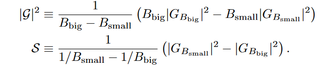
• Given estimates of $|G_{est}{|}^2$ for both $B=B_{small}$ and $B=B_{big}$, we can obtain unbiased estimates of $|\mathcal{G}{|}^2$ and $\mathcal{S}$ for $|G{|}^2$ and $tr(\Sigma )$, respectively
  • 
• We can compute $|G_{B_{small}}{|}^2$ and $|G_{B_{big}}{|}^2$ for free in a data-parallel method by computing the norm of the gradient before and after averaging between devices :)))
• Note that $|\mathcal{G}{|}^2/\mathcal{S}$ is not an unbiased estimator of ${\mathcal{B}}_{simple}=\frac{tr(\Sigma )}{|G{|}^2}$
  • Thus, we keep an EMA of both values such that the ratio of the moving averages is a good estimator of the noise scale.