Dealing with weights and activations

Quantization of the weights is performed using either symmetric or asymmetric Quantization.
Quantization of the activations, however, requires inference of the model to get their potential distribution since we do not know their range.
- There are two forms of quantization of the activations:
  - Dynamic Quantization
  - Static Quantization

Dynamic quantization

After data passes a hidden layer, its activations are collected:
This distribution of activations is then used to calculate the zeropoint (z) and scale factor (s) values needed to quantize the output:
The process is repeated each time data passes through a new layer. Therefore, each layer has its own separate z and s values and therefore different quantization schemes.

Similar to dynamic quantization but the $s$ and $z$ values are computed offline using a calibration dataset.

Based on the observation that only certain activation layers (e.g. residual connections after FFN) in BERT cause big performance drop, Bondarenko et al. (2021) adopted mixed-precision quantization by using 16-bit quantization on problematic activations but 8-bit on others.
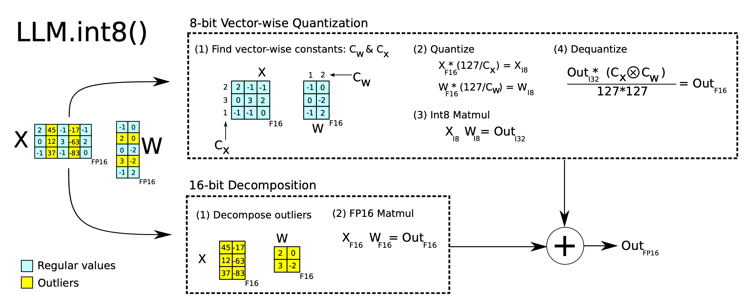
Mixed-precision quantization in LLM.int8() (Dettmers et al. 2022) is implemented via two mixed-precision decompositions:

Because matrix multiplication contains a set of independent inner products between row and column vectors, we can impose independent quantization per inner product: Each row and column are scaled by the absolution maximum values and then quantized to INT8.
Outlier activation features (e.g. 20x larger than other dimensions) remain in FP16 but they represent only a tiny fraction of total weights. How to identify outliers is empirical.

Naively quantizing the entire weight matrix in one layer (“per-tensor” or “per-layer” quantization) is easiest to implement but does not lead to good granularity of quantization.
Q-BERT (Shen, Dong & Ye, et al. 2020) applied group-wise quantization to a fine-tuned BERT model, treating an individual matrix with respect to each head in MHSA (multi-head self-attention) as one group and then applies Hessian based mixed precision quantization.
- Per-embedding group (PEG) activation quantization was motivated by the observation that outlier values only appear in a few out of (hidden state / model size) dimensions (Bondarenko et al. 2021).
- Per-embedding is pretty computationally expensive. In comparison, PEG quantization splits the activation tensor into several evenly sized groups along the embedding dimension where elements in the same group share quantization parameters.
- To ensure all outliers are grouped together, they apply a deterministic range-based permutation of embedding dimensions, where dimensions are sorted by their value ranges.
ZeroQuant (Yao et al. 2022) uses group-wise quantization for weights, same as in Q-BERT, and token-wise quantization for activation.
- To avoid expensive quantization and de-quantization computation, ZeroQuant built customized kernel to fuse quantization operation with its previous operator.

Q-BERT (Shen, Dong & Ye, et al. 2020) developed Hessian AWare Quantization (HAWQ) for its mixed-precision quantization.
- The motivation is that parameters with higher Hessian spectrum (i.e., larger top eigenvalues) are more sensitive to quantization and thus require higher precision. It is essentially a way to identify outliers.
GPTQ (Frantar et al. 2022) treats the weight matrix as a collection of row vectors and applies quantization to each row independently.
- GPTQ iteratively quantizes more weights that are selected greedily to minimize the quantization error. The update on selected weights has a closed-form formula, utilizing Hessian matrices.
- Read more details in the paper and the OBQ (Optimal Brain Quantization; Frantar & Alistarh 2022) method if interested.
- GPTQ can reduce the bitwidth of weights in OPT-175B down to 3 or 4 bits without much performance loss, but it only applies to model weights not activation

It is known that activations are harder to quantize than weights in transformer models.
SmoothQuant (Xiao & Lin 2022) proposed a smart solution to smooth outlier features from activations to weights via mathematically equivalent transformation and then enable quantization on both weights and activations (W8A8).
- Because of this, SmoothQuant has better hardware efficiency than mixed-precision quantization.
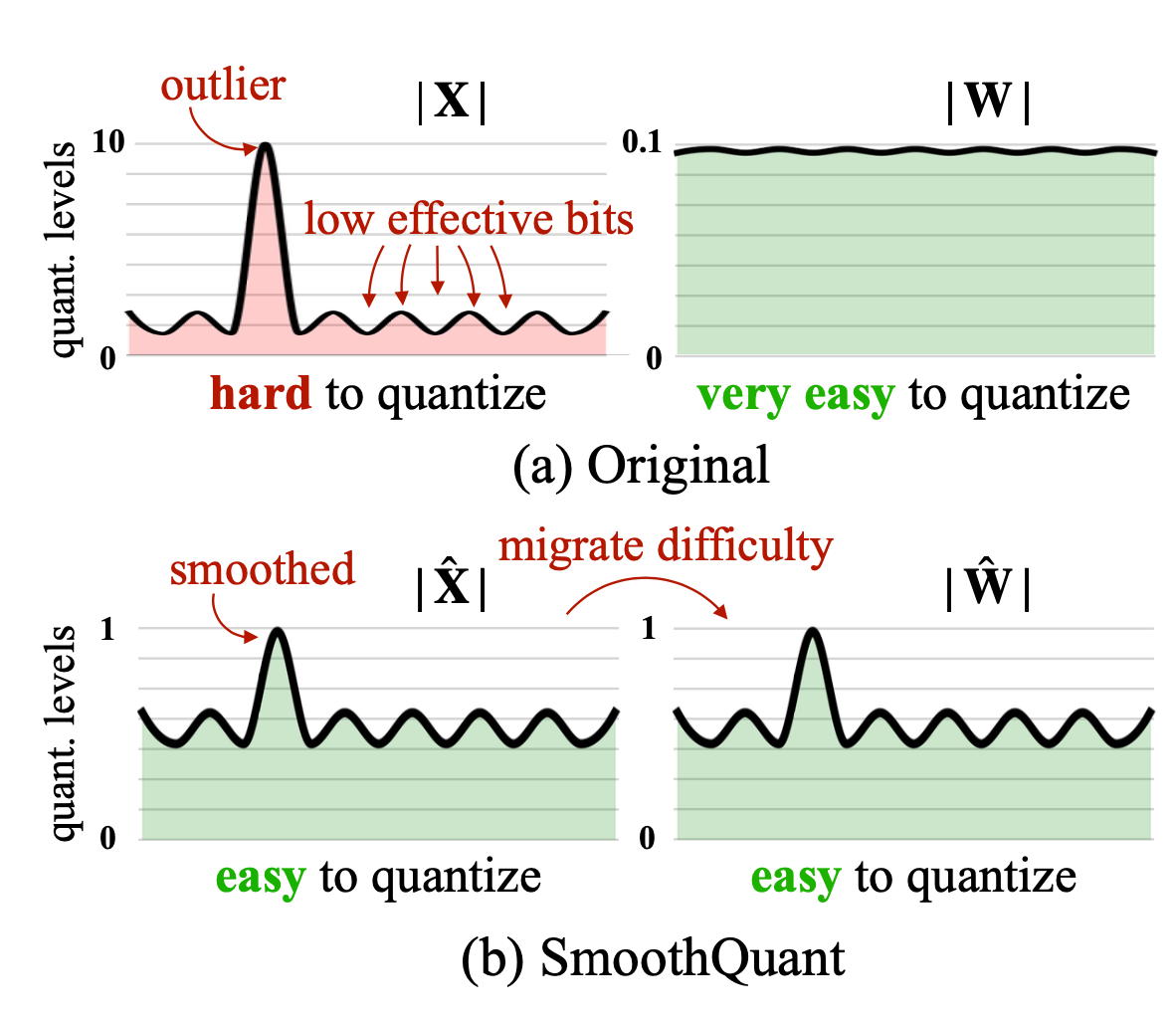
- SmoothQuant migrates the scale variance from activations to weights offline to reduce the difficulty of activation quantization. Both the resulting new weight and activation matrices are easy to quantize.
- Considering a per-channel smooth factor $s$ , SmoothQuant scales the weights according to:
  - $Y = (X diag (s)^{- 1}) \cdot (diag (s) W) = \hat{X} \hat{W}$
  - The smoothing factor can be easily fused into previous layers’ parameters offline.
    - A hyperparameter $α$ controls how much we migrate the quantization difficulty from activations to weights: $s = max (∣ X_{j} ∣)^{α} / max (∣ W_{j} ∣)^{1 - α}$ . The paper found that $α = 0.5$ is a sweet spot for many LLMs in the experiments. For models with more significant outliers in activation, can be adjusted to be larger.