u-mup

• u-μP: The Unit-Scaled Maximal Update Parametrization

Summary

• u-μP, which improves upon μP by combining it with Unit Scaling:
  • μP ensures that the scale of activations is independent of model size
  • Unit Scaling ensures that activations, weights and gradients begin training with a scale of one.

Detailed

• you need to divide the residual add to prevent the model from blowing up

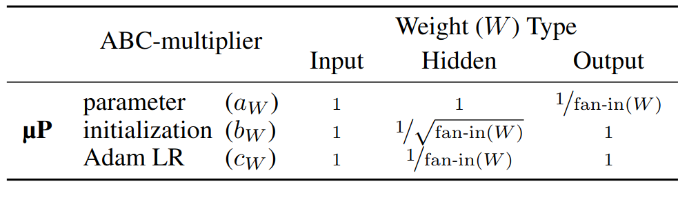
Reminder of mup setting

ABC-parametrization

• ABC-parametrizations μP, SP, and the Neural Tangent Kernel (NTK) are all instances of abc-parametrizations. This assumes a model under training where weights are defined as:
  • $w_0\sim \mathcal{N}(0,B_W^2)$
  • $W_t=A_W\cdot w_t$,
  • $w_{t+1}=w_t+C_W\cdot {\Phi }_t(\nabla L_0,...,\nabla L_t)$,
  • with $t$ a time-step and ${\Phi }_t(\nabla L_0,...,\nabla L_t)$ the weight update based on previous loss gradients.
• $A_W$ = parameter multiplier
  • For example, in the attention logit calculation $⟨k,q⟩/\sqrt{d_{head}}$ where $q=Wx$, the $1/\sqrt{d_{head}}$ factor is a multiplier. It may also be thought of as the parameter multiplier of $W$ if we rewrite the attention logit as $⟨k,(W/\sqrt{d_{head}})x⟩$.
  • Note that parameter multipliers cannot be absorbed into the initialization in general, since they affect backpropagation. Nevertheless, after training is done, parameter multipliers can always be absorbed into the weight.
• $B_W$ = per-parameter initialization
• $C_W$ = per-parameter learning rate
• A parametrization scheme such as μP is then defined specifying how scalars $A_W$ , $B_W$ , $C_W$ change with model width.
  • This can be expressed in terms of width-dependent factors $a_W$, $b_W$, $c_W$, such that $A_W\propto a_W$, $B_W\propto b_W$, $C_W\propto c_W$.
  • (The scaling defining mup)

ABC-symmetry

• A key property of the abc-parametrization is that one can shift scales between $A_W$, $B_W$, $C_W$ in a way that preserves learning dynamics (i.e. the activations computed during training are unchanged). We term this abc-symmetry. For a fixed $\theta >0$, the behavior of a network trained with Adam is invariant to changes of the kind: $A_W\leftarrow A_W\cdot \theta ,B_W\leftarrow B_W/\theta ,C_W\leftarrow C_W/\theta$
  • This means that parametrizations like $\mu P$ can be presented in different but equivalent ways. ABC-symmetry is a key component in developing u-$\mu P$. (and why the u-mup scheme is consistent mup and Spectral mup)

Transferable HPs

• The above terms are defined by the parametrization choice, however there are also the hyperparameters chosen by the user.
• All μTransferable HPs function as multipliers and can be split into three kinds, which contribute to the three (non-HP) multipliers given by the abc-parametrization: ${\alpha }_W$, ${\sigma }_W$, ${\eta }_W$ where $A_W\propto {\alpha }_W$, $B_W\propto {\sigma }_W$, $C_W\propto {\eta }_W$.
• ${\alpha }_W$ = operator scaling
• ${\sigma }_W$ = init scaling
• ${\eta }_W$ = per-parameter learning rate scaling

The challenges with mup in practice

• Not all training setups give mu-Transfer

  • Vanilla mup works in overfitting regime but fails to generalize to standard LM training regime (under-fitting)
  • The fix is (1) Removal of trainable parameters from normalization layers (2) Use the independent form of AdamW Independent weight decay

• It’s not clear which hyperparameters to sweep

  • In theory, the search space of μTransferable HPs includes ${\alpha }_W$, ${\sigma }_W$, ${\eta }_W$ for every parameter tensor W in the model
  • there’s coupling between them if you’re not careful
    • The relative size of a weight update is determined by the ratio ${\mu }_W/{\sigma }_W$ (size of update / size of current weight)
    • Consider the commonly-used global ${\sigma }_{init}$ HP. At initialization the activations going into the FFN swish function have $std(x_{swish})\propto {\sigma }_{W_{gate}}$, whereas the self-attention softmax activations have $std(x_{attn})\propto {\sigma }_{W_Q}{\sigma }_{W_K}$. A global $\sigma$ HP thus has a linear effect on the FFN and a quadratic effect on attention, suggesting that this grouping may not be ideal.

• Base shape complicates usage

  • Orignal mup requires an extra “base” model to correctly init the model

• mup struggles with low-precision

  • Low-precision training runs succesfully converging in SP can diverge with mup because of the generally lower init and scaling (underflow of gradients)

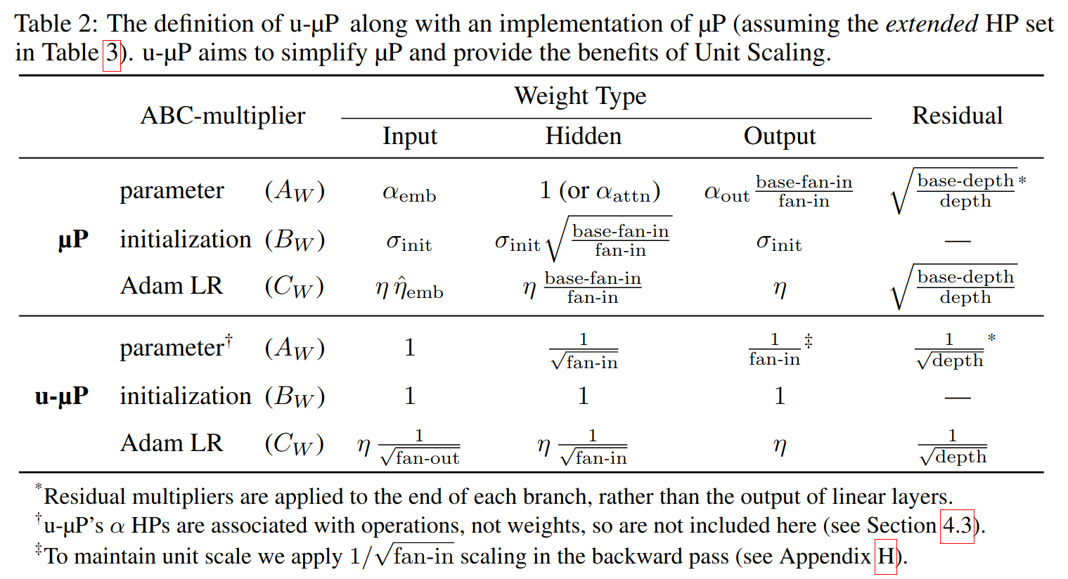
The Unit-Scaled Maximal Update Parametrization

The u-mup ABC parametrization

• 

• How they go from mup to u-mup

  • drop the ${\sigma }_W$ (because unit scaling assumes unit variance)

    • they can do so by using ABC-parametrization to shift the scale in $B_W$ (i.e. the $\frac{1}{\sqrt{fan-in}}$) from mup to $A_W$ and $C_W$ (Equation 4 and 5 in the paper)

  • drop the $\mathrm{base}-\mathrm{fan}-\mathrm{in}$ HP with the above trick and also shifting the ${\alpha }_W$ HPs burden to the unit scaling ops

  • change the input learning rate to $1/\sqrt{fan-out}$.

    • slight deviation for mup in terms of the math
    • key change for performance, not much theoretical justification

• It’s important to note that the scaling rules in this table must be combined with the standard Unit Scaling rules for other non-matmul operations.

  • e.g. gated SILU, residual_add, softmax cross-entropy, …

Why it works better than vanilla mup

• We can attribute the difficulties μP has with low precision to the fact that it ignores constant factors (along with weight and gradient-scaling), only ensuring that activations are of order $\Theta (1)$. The stricter condition of unit scale across all tensors at initialization provides a way of leveraging μP’s rules in order to make low-precision training work.

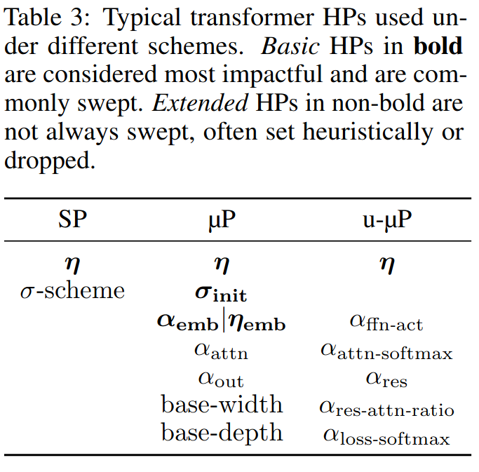
A principled approach to hyperparameters

• How to sweep HPs has been a mess in mup literature
• We want
  • Minimal cardinality: the use of as few HPs as possible.
  • Minimal interdependency: the optimal value of each HP should not depend on the value of other HPs, simplifying the search space.
  • Interpretability: there should be a clear explanation for what an HP’s value ‘means’ in the context of the model

1. we can drop all ${\sigma }_W$ as we assume unit scaling (and abc-symmetry allows us to do so), leaving just ${\alpha }_W$ and ${\eta }_W$
2. Second, several ${\alpha }_W$ combine linearly with other ${\alpha }_W$ HPs. It is easier to define things at the operator level instead of the weight level, e.g. $std(x_{attn})\propto {\alpha }_{W_Q}{\alpha }_{W_K}$. In this instance, it is more natural to use a single $\alpha$ parameter and associate it with ${\alpha }_{attn-softmax}$
3. Use a single global $\eta$ and group $\alpha$ HPs across layers. (This is the best tradeoff between expressivity and cardinality)

• The considered hyperparameters for a Transformer

  • 

• How to choose such operator multipliers for an architecture is described in Appendix F and Appendix G

  • The idea is that you want a multiplier at every operation in your computational graph where there’s a non-homogeneous function or a non-unary function (not single input)
    • i.e. a k-homogeneous function is $h\to f(h)$ s.t. $f(\alpha h)={\alpha }^{k}f(h)$
    • RMS norm is 0-homo., Linear is 1-homo. and QK matmul is 2-homo.
    • A residual add is non-unary
    • Sigmoid and cross-entropy loss is non-homogeneous
  • After having settled on needed multipliers, simplify them following the minimal cardinality, expressivity, and interpretability constraints
    • assuming unit-scaling usually allows for more interpretable mutlipliers

How to do the HPs sweep

• The standard approach to HP search for mu-Transfer is via random sweep over all HPs simultaneously. This is costly

• Due to the inter-dependence criterion applied previously, u-mup supposedly allows for a simpler scheme, called independent search

• The idea is to first sweep the LR, followed by a set of one-dimensional sweeps of the other HPs (which can be run in parallel). The best results from the individual sweeps are combined to from the final set of HP values.

• The simpler scheme, which only sweeps the LR, leaving other HP values at 1, seems to work well in practice.

Numerical properties

• mup has gradients and weights with low RMS, at risk of FP8 underflow, whereas u-μP starts with RMS ≈ 1.

• Many input activations do not grow RMS during training (due to a preceding non-trainable RMSNorm), however the attention out projection and FFN down projection have unconstrained input activations that grow considerably during training

• The decoder weight grows during training. Since it is preceded by a RMSNorm, the model may require scale growth in order to increase the scale of softmax inputs. Other weights grow slightly during training.

• Gradients grow quickly but stabilize, except for attention out projection and FFN down projection, whose gradients shrink as the inputs grow.

• The the main parameter affecting scale growth is learning rate

  • End-training RMS is remarkably stable as width, depth, training steps and batch size are independently increased.

Prerequisites before applying u-mup

• Remove trainable parameters from normalization layers
• Use the independent form of AdamW Independent weight decay
• Ensure training is the under-fitting regime (i.e. avoid excessive data repetition)

A guide to using u-mup

• Being careful of tensors with scale growth (inputs to FFN and self-attention final projections)
  • use E5M2 format to represent the larger scales or apply dynamic rescaling of the matmul input
• apply unit scaling with the correct scale constraints, for new operations, don’t hesitate to fit an empirical model for the scale of the op.

Hyperparameter transfer results

• The setting matters a lot (i.e. number of tokens, model size, sequence length). Should be as representative as possible of the final training.
• At large scale, learning rate $\eta$ and residual attention ratio ${\alpha }_{res-attn-ratio}$were the most important HPs. All other HPs can be left at their default value of 1.
• Non-LR HPs also have approximately constant optima across width under u-μP

How to use a good proxy model

• When using a relatively small proxy model with 8 layers and a width of 512 (4 attention heads), the HP-loss landscape is rather noisy. By doubling the width, they are able to discern the optimal values of the HPs more clearly.
• In general, width is the most reliable feature to transfer. Training steps and batch size also give good transfer, so moderate changes here are permissible. Depth is the least reliable feature for transfer, so they only recommend modest changes in depth
• Keep the number of warmup steps constant, but always decay to the same final LR when varying the number of steps.